Lecture 9-1 - Sorting, Searching, Success

You’re sitting here, in a computer science course, and wondering: why the hell am I getting all of this education just to learn how to sort things?

Well, probably because you’ve been sorting things poorly your whole life!

More accurately, because you need to know how to sort data efficiently for a wide breadth of applications, and analyzing these sorting algorithms gives us some good practice with our new tools from asymptotic runtime analysis.

Question

What are some applications of programmatic sorting that you can think of?

Answer

To name a few:

• Any tables with data that allow for filters (e.g., Excel can sort rows by the values in a particular column)
• Web pages returned by a search engine ranked by relevance
• Too many others to list!

Throughout the next part of this class, we’ll examine a variety of sorting algorithms and learn that some are better suited for some sorting tasks than others.

For now, we’ll start (as always) with some definitions and preliminaries…

Preliminaries

Definition

Sorting involves the act of ordering items in a collection systematically according to some sorting criteria.

Example

Example criteria include “least to greatest number” or “earliest alphabetic last name to latest”

The systematic aspect of sorting has been of research interest for computer scientists since the dawn of the digital age, and many algorithms have sprung forth from such endeavors.

Not only are there different sorting algorithms, but also different categories of sorting algorithms. We’ll look at the simplest today:

Definition

Comparative sorting algorithms sort elements in a list by using basic comparison operations (such as “greater than” or “less than or equal to”) to order elements in the final, sorted list.

Definition

Comparative sorts typically apply to Lists as the ADT of choice, but different sorting algorithms may be more amenable to ArrayLists due to their capacity for Random Access.

We’ll now examine a typical comparative sorting algorithm, see how they work, what they’re good at, and what they’re horrible at.

Insertion Sort

Definition

Insertion sort is typically referred to as the “card sorting” algorithm, since it emulates how humans sort playing cards by selecting one and then dropping it into its sorted place in the hand.

Remark

Intuition: sort sublists of size i from the original list from index [0, i-1], “sliding” in the next int at i into its proper spot to the left!

The second most cliche sorting algorithm, insertion sort operates with the following steps:

1. Start at the left-most item, and look at the sub-list of 1 item, then 2, then 3, etc.
2. Iteratively grow the sublist, adding the next indexed item to its end, then “sliding” it into its proper position to the left so that the sublist is now sorted.
3. Repeat until the sublist is the original list (i.e., consists of the same items).

Formally, the pseudocode of the algorithm that accomplishes the above is as follows:

// Sort sublists from the start of size i
for each element i in the array, starting with i = 1:
    // At the start of this inner loop, everything from index [0, i-1]
    // will be sorted, so see where the int at index k should go!
    for each element k = i down to k = 1 where arr[k] < arr[k-1]:
        swap a[k] and a[k-1]

So, the idea is that we continue to lock items at the front of the array into their proper place, assuming everything to the left of the current one is sorted already.

Example

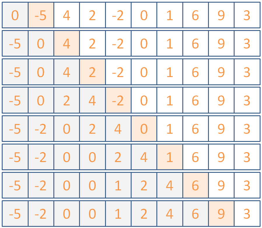
Use Insertion Sort to sort the following list of ints:

Question

Click here for the steps the algorithm would take.

Answer

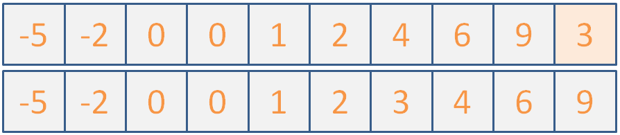
(maybe if I don’t say anything, they won’t notice that the illustration is actually two different images because I couldn’t fit it all into one slide…)

Any who, let’s implement this now; it won’t take long!

Example

Complete the shell for InsertionSort below:

// ...
 
private void swapIntsAt (int index1, int index2) {
    int temp = items[index1];
    items[index1] = items[index2];
    items[index2] = temp;
}
 
public void insertionSort () {
    // [!] Iterate through each element of the array
    // starting with i = 1
    for ( ??? ) {
 
        // [!] Starting at index i, examine pairs
        // of ints moving down to (and including)
        // index 1
        // AND
        // only swap ints if the currently
        // examined element is less than the one
        // before it in the list
        for ( ??? ) {
            // [!] If we're in the loop, it means that
            // we need to swap the two adjacent ints
            // (otherwise, they were already in order and
            // we never entered this loop)
            this.swapIntsAt( ??? );
        }
    }
}
 
// ...
 
public static void main(String[] args) {
    IntArrayList listy = new IntArrayList();
    listy.append(5);
    listy.append(2);
    listy.append(1);
    listy.append(4);
    listy.append(3);
    System.out.println("Pre-sort:  " + listy);
    listy.insertionSort();
    System.out.println("Post-sort: " + listy);
}

Question

Click for solution…

Answer

public void insertionSort () {
    // Sort sublists from the start of size i
    for (int i = 1; i < this.size; i++) {
        // At the start of this inner loop, everything from index [0, i-1]
        // will be sorted, so see where the int at index k should go!
        for (int k = i; k >= 1 && this.items[k] < this.items[k-1]; k--) {
            swapIntsAt(k, k-1);
        }
    }
}

Runtime Performance of InsertionSort

Having seen it implemented, let’s think about the performance of InsertionSort, including how we might use our new asymptotic notation to characterize it.

Firstly, let’s think about what type of an algorithm InsertionSort represents:

Definition

InsertionSort is a type of algorithm known as a “reduce-and-conquer” / “decrease-and-conquer” because they incrementally decrease the size of the problem into smaller ones, or start with small problems that are incrementally increased until the original problem is solved.

However, the amount of work done within one of those incrementally developing subproblems can be different depending on some characteristics of the task at hand.

Remark

In particular, with using InsertionSort on a list of items, there are some characteristics of how the list’s data is arranged in the pre-sort condition that might make a performance difference!

Toolkit

For this reason, asymptotic performance analysis is often performed under assumptions of the problem’s Best, Worst, and Average Case.

Let’s think about what those cases are for InsertionSort.

Question

Best Case: Starting with the easiest question: what is the Best Case for InsertionSort (i.e., when will it take the fewest steps?) and what will its asymptotic runtime complexity be in this scenario?

Answer

When the list is already sorted (or almost so)! In this case, the inner loop is essentially constant time O(1) repeated n times to verify that it is sorted, giving us: O(n).

The interesting thing with the best case is that even though there’s little-to-no swapping of items done, there’s still a linear cost associated with the verification that the list is indeed sorted.

Slightly less easy, however, is for the Worst Case, whose analysis relies on some keen insights:

• The inner loop relies on the current value of the outer loop
• Since we’re always going to run through the outer loop all n times, we need to find the characteristics of the list that will maximally run the inner loop.

With those insights made…

Question

Worst Case: What is the Worst Case for InsertionSort (i.e., when will it take the most steps?) and what will its asymptotic runtime complexity be in this scenario?

Answer

The answere here has some subtlety. Firstly, we note that the worst case is when we have to make the maximal number of swaps, meaning the list begins in reverse-sorted order.

As such, to determine its complexity in this scenario, we could write the number of steps that it would take in the inner loop as a function of the outer loop’s value for i. This means that, again in the worst case, we take 1 step to swap when i = 1, 2 steps when i = 2, etc. etc. So, we can be clever and write:

// Let L_i = the number of steps taken inside the
// inner "swapping" loop at iteration i of the outer
T(n) = L_1 + L_2 + L_3 + ... + L_{n-3} + L_{n-2} + L_{n-1}
     = 1 + 2 + 3 + ... + (n - 2) + (n - 1) + n
     // We can re-write the above as some number of (n+1) terms... how many?
     = (n + 1) + (n + 1) + ... + (n + 1)
     // Well, n/2 of them! Because we're pairing them up
     = (n/2) * (n + 1)
     = (1/2) * (n^2 + n)
     = O(n^2)

With the Best and Worst Cases diagrammed, we see that there’s a lot of wiggle-room when it comes to the performance of InsertionSort! The difference between linear and quadratic runtimes is severe (as we’ve seen from the ArrayList prepend debacle).

That said, we should make an observation for the Average Case performance here as well. In general, arguing for the Average Case must be done formally through some sort of proof which may even examine empirical likelihoods of distributions over the data. For us, let’s just do some intuiting…

Question

Average Case: What is the Average Case for InsertionSort (i.e., what does the typical task look like?) and what will its asymptotic runtime complexity be in this scenario?

Answer

(Sketched Answer): We can imagine that, in the average case, there will be roughly 1/2 the numbers that are “easy” to sort (i.e., nearly in place) and 1/2 that are “harder” (i.e., not near their proper place). This gives us an easy average case performance of (O(\frac{n}{2} + \frac{n^2}{2}) = O(n^2))

Example

There are some good InsertionSort animations located here. Which properties of data does InsertionSort excel at sorting? With which properties does it struggle?

Later in the course, we’ll not only gain the tools for analyzing the performance of these sorting algorithms, but find alternatives that are generally faster and more robust to variant properties of the data.

For now, onto a different task!

---

Membership Search

Let’s take a look at a relevant operation that exposes a different computational complexity class compared to what we’ve thusfar seen.

The motivation: examining the membership search operation upon some list of elements.

Preliminaries

Definition

Membership Search algorithms determine if a collection contains one or more elements according to some criteria.

This is pretty much exactly like it sounds: you have some collection and you want to know if something is among its elements.

Question

What are some metrics of success for a search operation?

Answer

1. Completeness: that it will find the query if it exists or conclude otherwise; 2) Efficiency: that the search will complete with as few steps as possible.

So, let’s consider the task of finding a number from a List of integers.

Example

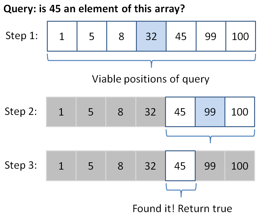
Trace the steps of determining whether or not the number 45 exists in the List: [1, 5, 8, 32, 45, 99, 100]

Now, humans have a fairly easy time searching for an item in a list, especially one that is small.

But, let’s consider how a program might handle the operation.

Question

Assuming we used a brute-force approach starting at the front of the list, how many steps would it take to find 45?

Answer

5 steps, since we would iteratively check if each element is contained in the list.

Question

What is the asymptotic runtime complexity of this elementary search operation for a list of size n?

Answer

O(n), since we must examine each element linearly in the list.

A linear search isn’t terrible, but perhaps we can do better…

Binary Search

Remark

Notice something about our example array: its elements are sorted in ascending order!

Question

Can we take advantage of a sorted list to somehow improve our search over the linear case?

Answer

Yes, because we know that everything to the left of an element will be less than it, and everything to the right will be greater.

This means that if I’m searching for a particular item in a sorted List, I don’t need to look at every item to determine if it’s contained within!

Definition

Binary search is a search algorithm that exploits sorted data structures by excluding portions of the search space as viable locations for the query.

The algorithm for implementing binary search for a List is fairly simple:

1. Start by examining the element at the middle index.
2. If it is your query, you’re done, otherwise:
   • If your query is less than the examined element, then repeat from step 1 on the left half of the list.
   • If your query is greater than the examined element, then repeat from step 1 on the right half of the list.

Let’s see how that looks:

Question

How many steps did our binary search on this list take?

Answer

3 steps! An improvement over our linear search.

However, the asymptotic complexity of binary search might surprise you (clickbait sentence lol).

Question

With every step of binary search, how much of the search space is removed from consideration?

Answer

Half, since we know that if the query exists somewhere in the list, it must be on one side of the middle or the other.

So, if at every step we’re reducing the search space by half until we find our query, what is the asymptotic growth rate of binary search?

Definition

Binary search has a logarithmic growth rate, indicated by O(log(n)).

For those who might be unfamiliar with logs, they are essentially the dual of exponentiation. Here’s the anatomy of a log:

Toolkit

The log_b(n) = p notation means that if we raise base (b) to the power (p) then we get the number, n.

Example

Here are some example logarithms:

log_2(8)    = 3   // because 2^3  = 8
log_10(100) = 2   // because 10^2 = 100

So, let’s consider how logs relate to the complexity of binary search.

Since we’re splitting the search space (of n elements) into 2 with each step, we are with each comparison essentially “undoing” an exponentiation of the search space.

In other words, if I have 8 elements, and am using binary search, then I need at most 3 steps to find an element (the first reduces the search space to 4, then to 2, then to 1 element).

This behavior is cleanly represented in the logarithm, which we could write as:

// Applied to algorithmic growth rates:
log_{factor of split}({number of elements}) = {number of steps}

In terms of Big-O orderings, logarithmic growth is far superior to linear, thus giving us the updated ordering (from the growth rates we’ve seen) of:

Toolkit

O(1) < O(log(n)) < O(n) < O(n*log(n)) < O(n^2)

Binary search will help us construct some data structures to come, but for now, we’ll keep it in our back pocket as an illustration of a new, interesting computational complexity class.

---