In the previous section, we began noticing that the performance between certain operations on certain data structures could be different depending on the scenarios in which
they were used. (wow what a vague sentence)
For instance: we say that prepending data to a linked list was less computationally expensive than prepending data to a sequential one.
We’ll now start to formally characterize performance differences between different algorithms and the data structures they employ.
Empirical Analysis
Once again, in the previous section, we timed how long it took for a sequential list to prepend a couple million items vs. a linked list, and saw that linked lists took far less time.
Question
Is this an objective method of comparing the run-times of different algorithms? If not, what factors might not make it objective?
Answer
No, this is not an objective metric for the following reasons:
Running algorithm 1 at 2:59 and algorithm 2 at 3:00 (when you happened to, say, have your virus scan scheduled) can impact runtime for shared computer resources!
Running compared algorithms on two different computers can have mixed-sample results because of differences in hardware (e.g., multiple processors on one computer
but not another), operating systems, etc.
What if your test happened to be the best case operating scenario for algorithm 1, but the worst case for algorithm 2? What if another test with changed input
would have been the best case for algorithm 2 instead? Which test should you run? Can you just average the results of both? Well then what if there’s a 3rd test… etc.
For these reasons, we need a more objective means of being able to evaluate our algorithmic performance that is invariant to the above.
Example
Suggest some alternative means of objectively evaluating algorithmic performance.
Performance Analysis - Objectives
As it turns out, the CS powers that be decided on a now well-established analytic system:
Definition
Run-time / Performance Analysis provide a theoretical classification of the running time of a particular
algorithm (the number of primitive operations or “steps” required) as a function of its input size.
Note: “Input size” is a general term that usually refers to one of the following: the size of some value entered by a user or the number of elements in a particular
data structure.
Definition
Run time analysis considers the growth rates in the number of steps that an algorithm takes as the size of its input increases
(theoretically to infinity).
Question
Why do we care about the run time of algorithms for huge inputs rather than smaller ones?
Answer
The answer is practical: (1) modern computers are so fast at executing algorithms for small inputs that the tangible performance differences
are usually only noticed for a large scale of data. (2) We also want a way to forecast how the algorithm were perform if the input continues to get larger.
Furthermore, to avoid any of the issues of empirical analysis as detailed in the previous section, we typically make a couple of hardware assumptions:
The Uniform Cost assumption states that every atomic machine operation (like addition) takes the same amount of time.
The Single Processor assumption states that we have a single processor that executes instructions in a linear fashion (i.e., no parallel execution).
We will formalize the metrics of performance analysis in a future lecture, but for now, let’s generate a little intuition…
Problem Complexity
We should be careful to distinguish between the performance of a given solution / approach / or algorithm in pursuit of solving a given problem, and the inherent difficulty of the problem
that we are attempting to solve.
This distinction is typically made in what is known as a problem’s complexity vs. the performance analysis of an algorithm that attempts to solve it.
Definition
The study of problem complexity is a field in CS theory that revolves around classifying computational problems according to their inherent difficulty,
and then relating / comparing those classes to one another.
Toolkit
Problem complexity will be the focus of your theory classes (Language & Autonoma I, II), but runtime complexity will be the focus of this one.
Let’s go through a famous example to drive the point home:
Example
Design an algorithm that accepts two integers, x and y, and returns their greatest common denominator (GCD).
A brute-force implementation might look like the following:
public class GCD { public static int gcd (int x, int y) { // For consistency's sake, we'll always make x the larger of x and y if (y > x) { int t = x; x = y; y = t; } // Handle simple cases immediately if (x == y || x % y == 0) { return y; } int currentGreatest = 1; for (int i = 1; i <= y; i++) { if (x % i == 0 && y % i == 0) { currentGreatest = i; } } return currentGreatest; } public static void main (String[] args) { System.out.println(gcd(10, 5)); // 5 System.out.println(gcd(5, 10)); // 5 System.out.println(gcd(2, 2)); // 2 System.out.println(gcd(2, 8)); // 2 System.out.println(gcd(4, 8)); // 4 System.out.println(gcd(21, 49)); // 7 System.out.println(gcd(1512, 1511)); // 1 }}
Question
Looking at the above implementation of gcd, what are (1) the best
case(s) for the number of steps the algorithm has to take, and
(2) how many steps does it take under these conditions?
Answer
The best cases are when x == y or y is already a factor of x. In these scenarios, the algorithm need only take 1 step!
Question
Looking at the above implementation of
gcd, what is (1) the worst case for
the number of steps the algorithm has to take, and (2) how many
steps does it take under these conditions?
Answer
The worst cases are when x != y, y is not a factor of x, and the two numbers have a gcd of 1 — this meant that we had to iteratively step through every number from 1 to y and verify that it
was not the gcd of x and y!
Definition
Typically, runtime analysis is contextualized by what cases of performance we’re analyzing. The three most common analyses take place for an algorithm’s worst, best, and average case
performances.
So, in the best cases, the answer is immediate… but otherwise, we could be making a huge number of comparisons! In gcd(1512, 1511), we’re already taking 1511 steps just to conclude that the answer is 1!
Thankfully, there’s a better algorithm for finding the gcd…
Toolkit
Euclid’s algorithm is a recursive approach to the gcd problem which stipulates that (for x > y) gcd(x, y) = gcd(y, r) if we express x = q * y + r for
x as some integer multiple q of y with remainder r.
Using the brute-force approach, how many steps would gcd(48, 20) have taken?
Answer
20, as we would need to loop through all factors to find the greatest.
Yet, using Euclid’s algorithm, we found the gcd in only 3 steps! Incredible!
It’s quite simple to implement the above:
public class GCD { public static int gcd (int x, int y) { // For consistency's sake, we'll always make x the larger of x and y if (y > x) { int t = x; x = y; y = t; } // Handle simple cases immediately if (x == y || x % y == 0) { return y; } return gcd(y, x % y); } public static void main (String[] args) { System.out.println(gcd(10, 5)); // 5 System.out.println(gcd(5, 10)); // 5 System.out.println(gcd(2, 2)); // 2 System.out.println(gcd(2, 8)); // 2 System.out.println(gcd(4, 8)); // 4 System.out.println(gcd(21, 49)); // 7 System.out.println(gcd(1512, 1511)); // 1 }}
Later, we’ll examine means of formally comparing the performances of these two algorithms, but the take-away points are as follows:
Finding the gcd of two numbers (as a problem) has its own class of complexity, and different algorithms that attempt to solve it will have their own performance complexities as well.
Problem and performance complexities might be different, though it’s generally the case that when they’re the same, you’ve found the optimal solution.
In this class, the important distinction will be classifying performances, comparing them, and being able to determine which are better solutions than others.
In particular, certain data structures will facilitate performance guarantees on different tasks… more to come!
Runtime Analysis
Last lecture, we now notice that the performance between certain operations on certain data structures could be different depending on the scenarios in which
they were used. (wow what a vague sentence)
For instance: we say that prepending data to a linked list was less computationally expensive than prepending data to a sequential one.
A reasonable question to now ask is: by how much better / worse will our performance benefit / suffer from the right / wrong choice of data structure?
Run-time Complexity
Remark
Just as we saw two different algorithms for the GCD problem (brute force and Euclid’s), and witnessed their drastically different performance, so too
will performance depend on choice of Data Structures.
Example
Let’s remind ourselves once more our comparison of the prepend operation in our array vs. linked lists:
import static org.junit.Assert.*;import java.util.*;import org.junit.Test;public class PrependTest { private static int TEST_SIZE = 200000; @Test public void testArrayListPrepend() { ArrayList<Integer> arr = new ArrayList<>(); for (int i = 0; i < TEST_SIZE; i++) { // [!] Adding i to index 0 = prepend operation arr.add(0, i); } } @Test public void testLinkedListPrepend() { LinkedList<Integer> arr = new LinkedList<>(); for (int i = 0; i < TEST_SIZE; i++) { // [!] Adding i to index 0 = prepend operation arr.add(0, i); } }}
Example
Tinker with the TEST_SIZE variable and plot: how much time does each test take as a function of the TEST_SIZE? Does it double for each data structure
if you double the TEST_SIZE? Plot n, the TEST_SIZE, and T(n), the time of each operation as a function of n.
Definition
This is precisely the task of run time analysis: to provide a means of characterizing the order of growth of the number of steps
an algorithm takes to complete as a function of the input size.
Plainly there is some non-linear relationship between the number of prepends we wish to make, and that operation in an ArrayList.
Since we don’t want to rely on empirical analysis to assign some runtime complexity to these operations, we’ll need to instead analyze the source code itself.
Analyzing Source
To summarize, we know a few punchlines about run time analysis thus far:
We want to be able to analyze an algorithm from the source code itself, thus side-stepping issues from empirical comparison.
We’re only interested in analyzing scenarios with big input size (i.e., trending to infinity).
We want to somehow characterize the growth rate of the number of steps an algorithm takes for this huge input.
Let’s start by discussing how we can analyze source code.
Toolkit
Primitive operations are those that take some constant number of steps to execute. We call this constant cost
(c_i) for some cost (c) associated with some statement (i).
Remark
Intuition 1: Primitive actions in most languages are those associated with the language-provided operators, or for simple getter methods that merely
return a value without the need for further computation, iteration, or any real effort.
Here are some example primitive operations in Java:
int i = 5;
if(i < 10)
System.out.println(i); (when we print out primitives like ints)
…
For students in computer systems organization, we recognize that each of these statements is composed of some number of machine instructions, but that these are constant for each
comparison or assignment or other simple operations.
Remark
Intuition 2: Different statements may take different amounts of time to execute, i.e., (c_i \ne c_k) but we’ll assume that each statement takes
the same amount of time every time it runs (not true for nondeterministic methods, but we won’t worry about those for now).
Toolkit
Then, the total time required for any algorithm to complete is indicated by (T(n)), the so called total cost function indicating the sum of all
individual time costs (c_i) in terms of n, the “size of the input” (that must be defined on a method-by-method basis).
T(n)=∑ici
Remark
Note that the total number of instructions executed will be proportionate to the actual (i.e., wall-clock) time it takes for some algorithm to execute!
This can be relatively straightforward, take the following code:
Above, we have a tiny algorithm that prints the ints on either side of the given int n.
Question
What is the total running time cost of nearestInts?
Answer
(T(n) = c_1 + c_2)
Question
Does the number of steps / amount of time required for nearestInts depend on the size of the input n? E.g., will it take a different number
of steps whether n is 1 vs. n is 10000?
Answer
No, notice that (n) doesn’t appear in the equation for (T(n)), so this algorithm takes the same number of steps regardless of what n is.
Definition
For this reason, we say that algorithms or statements whose run time is unaffected by the size of the input are said to
execute in constant time.
Example
Plot a constant time cost (T(n)) (y-axis) compared to growing n (x-axis).
So now let’s look at an algorithm that does depend on the size of the input.
Remark
Intuition 3: Algorithms employing iteration and recursion may have non-constant cost because individual statements’ costs (c_i) can be executed
multiple times as a function of the input size (n).
In such scenarios, we track not only the time cost c of a statement, but also the number of times it is executed.
public static void countTo (int n) { // Statements // Cost for (int i = 0; i < n; i++) { // c_1 * n System.out.println(i); // c_2 * n }}
Remark
Note: for conciseness, we’re using (c_1) to represent the sum of individual costs of int i = 0; (executed once so negligible) and then
(i \lt n; i++) repeated (n) times.
Question
What is the total running time cost of countTo?
Answer
(T(n) = c_1n + c_2n = n * (c_1 + c_2))
Question
Does the number of steps / amount of time required for countTo depend on the size of the input n?
Answer
Yes, notice we get another iteration from the loop every time we increment the input, n.
Notice also that (T(n)) features a factor with n on its RHS, indicating that the time it takes will change with the size of the input.
We also see that (T(n)) is a function that fits the equation of a line: (f(x) = ax + b). Here, we have (T(n) = (c_1 + c_2) * n + 0)
Definition
For this reason, algorithms or statements whose run time increases a near constant amount with every increase in the input size are said to be of
linear cost.
Example
Plot a linear time cost (T(n)) (y-axis) compared to growing n (x-axis).
WE HAVE TO GO DEEPER.
How about the following?
public static void countToInception (int n) { // Statements // Cost for (int i = 0; i < n; i++) { // c_1 * n for (int j = 0; j < n; j++) { // c_2 * n^2 // c_3 * n^2 System.out.println(i + " " + j); } }}
Question
What is the total running time cost of countToInception?
Does the number of steps / amount of time required for countTo depend on the size of the input n?
Answer
Yes, notice we get another iteration from the outer loop every time we increment the input, (n), and (n) more iterations from the inner loop!
Notice also that T(n) is a function that fits the quadratic equation: T(n) = ax^2 + bx + c (where c = 0).
Definition
For this reason, algorithms or statements whose run time increases a near linear amount with every increase in the input size are said to be of
quadratic cost.
Example
Plot a quadratic time cost (T(n)) (y-axis) compared to growing n (x-axis).
Composition
Thus far, we’ve operated under the assumption that our “atomic” operations like printing to output or instantiating a variable take some constant amounts of time, c_i.
However, because we’re scrutinizing source code, it’s important that we acknowledge operations that can ostensibly appear to take constant time, but actually take longer
in proportion to the size of the input.
Example
Scrutinize the following method f and write an expression for its run time as T(n) = T(arr.length).
...public static void g (int[] arr, int c) { // Cost for (int i = 0; i < arr.length; i++) { // c_3 * n System.out.println(c + arr[i]); // c_4 * n }}public static void f (int[] arr) { for (int i = 0; i < arr.length; i++) { // c_1 * n g(arr, arr[i]); // c_2 * n }}...
Well first off, the above is pretty useless (which is why the functions got generic names like f and g), but let’s look at something a little tricky.
Let’s examine specific parts of the above.
Question
Does the performance of f rely on the size of the input?
Answer
Yes, observe that c_1 is executed n times.
Question
Does the performance of g rely on the size of the input?
Answer
Yes, observe that c_3 is executed n times.
Question
What is T_g(n) = T_g(arr.length) for g?
Answer
T_g(n) = n * (c_3 + c_4)
Question
What is T_f(n) = T_f(arr.length) for f?
Answer
Observe that (T_f(n) = n * (c_1 + c_2)), but (c_2) is not a constant time operation. So, we will substitute its run time estimate appropriately:
T_f(n) = n * (c_1 + c_2)
       = n * (c_1 + T_g(n))
       = n * (c_1 + n * (c_3 + c_4))
       = n * c_1 + n^2 * (c_3 + c_4)
Takeaways from the above:
At first glance, f appears to have a linear runtime complexity until we scrutinize g as well, and realize that it is in fact quadratic.
Remember that only certain operations are considered to have constant run time as a function of the size of the input.
So, now that we’ve got a decent grasp for how to annotate specific lines of source code, let’s return to our original problem…
Asymptotic Analysis
Definition
Recall our original goal: to find an objective measure of the performance of two algorithms by comparing the growth in the number of steps taken
with an increase in the input size.
We’re about to reach this goal, but first, we need to see our solution’s motivation.
Motivation
Example
Suppose we compare two algorithms, a and b that perform the same operation but with different run-times.
We wish to compare the run times of these two algorithms to determine which is more efficient and find the following:
Assume (c_i) are all constant time operations but the precise amount of time is unknown
\begin{eqnarray}
T_a(n) &=& n^2 * c_1 \
T_b(n) &=& n * (c_2 + c_3)
\end{eqnarray}
Question
Can we tell, without knowing the magnitudes of (c_1, c_2, c_3), which algorithm is more efficient for arbitrary n? Why or why not?
Answer
Yes, but it may not be obvious why; for all we know, (c_1) might be massive compared to (c_2, c_3). We’ll examine how we can next…
Let’s unravel this a bit:
Example
Suppose we know (c_1 = 2) steps, (c_2 = 20), and (c_3 = 80). Compare (T_a, T_b) for (n = 10, 100, 1000).
n = 10
\begin{eqnarray}
T_a(10) &=& 10^2 * 2 &=& 200 \
T_b(10) &=& 10 * (20 + 80) &=& 1,000
\end{eqnarray}
A is the winner above for n = 10…
n = 100
\begin{eqnarray}
T_a(100) &=& 100^2 * 2 &=& 20,000 \
T_b(100) &=& 100 * (20 + 80) &=& 10,000 \
\end{eqnarray}
B is the winner above for n = 100…
n = 1000
\begin{eqnarray}
T_a(1000) &=& 1000^2 * 2 &=& 2,000,000 \
T_b(1000) &=& 1000 * (20 + 80) &=& 100,000
\end{eqnarray}
…and will continue being the winner ever onwards
Wow, there’s a lot to unpack from the above! Let’s make a couple of key observations:
Question
Observation 1: Algorithm a outperforms algorithm b for small n. Should we care about its early successes over b?
Answer
No, remember at the start of our discussion last week, we said that small n is inconsequential because modern computers can process these
smaller datasets very quickly. We do care about results as n trends to infinity.
So, to reiterate, we’re only interested in comparing performance for large n.
Furthermore, let’s examine the time costs of algorithm a more closely:
Observation 2: Which term “contributes” more to (T_a(n)): the (n^2) term, which depends on the input size, or the (c_1) term?
Answer
The (n^2) term. In fact, for large enough values of (n), the value of (c_1) becomes increasingly trivialized.
With these observations in mind, let’s combine them to devise a system to reach our goal: an objective measure of algorithm performance.
Asymptotics
Definition
Asymptotic runtime analysis provides a characterization of runtime performance as the size of the input, n, approaches infinity, i.e.,
limn→∞T(n)
This type of analysis is palatable because of our two observations above:
We only care about very large n, as n trends to infinity. Smaller n are trivialized because modern computers can quickly complete these operations.
The algorithm-subjective costs ((c_1, c_2), etc.) are numerically dominated by the number of times they are executed as a function
of the input size ((n, n^2), etc.)
Toolkit
It would be nice, then, if we could compare only the growth rate in steps an algorithm takes as a function of ever increasing n.
This is precisely what we’ll attempt to do, using asymptotic notation.
Definition
Asymptotic notation is a way of describing a set of functions (like (T(n))) that are bounded by another.
Definition
Asymptotic notation allows us to talk about equivalence classes of run time growth as n trends to infinity.
Remark
Thus, instead of talking about algorithm-subjective runtime functions (T(n)) (which are hard to compare), we can compare algorithms in terms
of growth classes of run time.
There are many ways to bound functions, but we’ll be examining one in particular, which describes a means of bounding a function above.
Big-O Notation
Definition
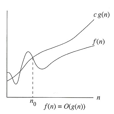
Big-O notation, written (T(n) = O(g(n))), says that (g(n)) is the asymptotic upper bound for (T(n)). In words,
“(T(n)) will never grow faster than (O(g(n)))” (up to some constant of proportionality).
Definition
Formally, written (T(n) = O(g(n))), says that (T(n)) shall never be larger than (c*g(n)) for some constant (c), after (n) has reached
some minimum value (n_0).
Remark
Intuitions:
(T(n)) is the total cost function we’ve been diagramming above, which is messy and hard to compare.
(g(n)) is some simpler “class” of (T(n))‘s performance for huge input.
(n_0) is just a starting point for the scaling of performance, since we don’t care about small (n) less than (n_0), just big inputs larger than it.
This might look, pictorially, like the following (stolen shamelessly from your textbook), where (f(n)) is a function like (T(n)):
Things to note about the above:
(f(n)) is bounded above by (c*g(n)) for any given c.
This bounding is only required to apply for n greater than n_0 (before which, the bounding did NOT hold, but is OK because we don’t care about small n).
Remark
Notes from Calculus: to find (T(n) = O(g(n))), generally just take the largest degree of (n) found in (T(n)) (i.e., the term with (n)
that has the highest exponent).
Example
Consider the following functions (T(n)) that describe the number of steps an algorithm takes, and for each, characterize its growth rate in Big-O notation.
// #1T(n) = 5 = O(1) - Explanation: O(g(n)) = O(1) says that T(n) = 5 will never be larger than c*g(n) for some constant c = 6 (or larger) after n = n_0 = 0. - When a function has O(1), we say it has a *constant* growth rate// #2T(n) = 5n + 6 = O(n) - Explanation: O(g(n)) = O(n) says that T(n) = 5n + 6 will never be larger than c*g(n) for some constant c = 10 after n = n_0 = 6. - When a function has O(n), we say it has a *linear* growth rate// #3T(n) = 3n^2 + 4n + 5 = O(n^2) - Explanation: O(g(n)) = O(n^2) says that T(n) = 3n^2 + 4n + 5 will never be larger than c*g(n) for some constant c after n = n_0. - When a function has O(n^2), we say it has a *quadratic* growth rate
Definition
(O(1), O(n), and O(n^2)) are ordered equivalence classes of run time growth rates, meaning that algorithms belonging to O(1) will
perform faster than those belonging to (O(n)), and those belonging to (O(n)) will perform faster than those belonging to (O(n^2)).
Toolkit
The best algorithms perform at (O(1)), but there are relative orderings of equivalent growth classes across many, many functions of n.
(O(n), O(n^2)) are two of the most commonly encountered classes, but there are others that we will see later as well! Just remember that (O(1)) is the best.
Big-O Rules of Thumb
Remark
Disclaimer: these are simply rules of thumb to start generating intuition for finding asymptotic performance guarantees. They are not exhaustively
applicable, but we will be considering exceptions explicitly later in the course.
For many algorithms, determining which run time growth class they belong to can be quite difficult and requires formal mathematical proofs.
For some basic ones, however, there are a few rules of thumb to find O(g(n)) from a given algorithm’s T(n).
Toolkit
If T(n) is a constant that does not depend on the input size, T(n) = O(1).
For example, T(n) = 5 = O(1) like in the example above.
This makes intuitive sense because an algorithm whose number of steps does not change with the input size will always take the same number of steps.
Toolkit
If T(n) contains factors that depend on the input size, then we may ignore the constant coefficients on terms with n.
In the above example #2, we had T(n) = 5n + 6 = O(n).
Using Observation 2 from the previous section, we see that the term 5n will dominate the number of steps this algorithm takes.
However, as n trends to infinity, the coefficient 5 plays only a tiny role, and so can be dropped entirely.
The +6 steps are even more trivial compared to a term where n is growing towards infinity, and so can be dropped as well.
So, dropping the +6 and the 5 coefficient from T(n) simply gives us O(n).
Toolkit
If T(n) contains factors that depend on the input size in different degrees, we may ignore all but the highest-order term.
For example, the degree(n^2) = 2 because it has a 2 for an exponent. The degree(5*n) = 1. The degree(5) = 0 because it is technically 5 * (n^0).
So, we say that the highest degree terms that rely on the size of the input dominate the other.
In the example #3 above, we had T(n) = 3n^2 + 4n + 5 = O(n^2).
Because 3n^2 is the highest order term, we ignore the others, and using our rule of thumb above, can ignore the 3 coefficient, giving us O(n^2).
Example
So, returning to our previous example, determine which algorithm is more asymptotically efficient:
(T_a(n) = O(n^2); T_b(n) = O(n)). (O(n) \lt O(n^2)), therefore algorithm b is asymptotically more efficient.
Big-O in Practice
Now that we’ve gleaned the theoretical underpinnings of run time analysis, let’s try it out in practice.
Before we do, consider one small fly in the ointment:
Question
Do all algorithms / DS methods perform with the same efficiency every time they’re called? If not, what is an example that we’ve seen of a
data structure performing differently based on differences in its state?
Answer
No, consider an ArrayList’s append; generally, this is a very quick operation… when there is room to append a new value!
Otherwise, we needed to perform the checkAndGrow procedure as a result.
So, how do we qualify our analysis if we can’t concisely determine the algorithm performance across input and state variants?
Definition
For most algorithms, run time analysis is performed for three separate input assumptions: (1) the worst case, (2) the average case, and (3) the best case.
The best and worst cases are generally easy to analyze: assume either the best or worst type of inputs and then determine which statements are executed more or less
in response to those types of inputs.
Average case analyses are more tricky and can often involve complex proofs to support their claims. We will not be detailing most of these proofs, but will still gain
some intuition for them.
Example
For the ADTs we’ve considered thusfar, provide runtime analyses for the best and worst cases of common operations like access, insertion, and removal.
Operation
Array Lists
Linked Lists
Arbitrary Retrieval
Insert / Remove from End
Arbitrary Insertion
Arbitrary Removal
Example
Bonus: what asymptotic complexity holds for operations of Queues and Stacks? (hint: they’re all the same!)
Amortized Time
Remark
Note a small asterisk we’ll attach to ArrayList insertion operations to account for the checkAndGrow procedure… but this doesn’t happen every time
we insert a new element!
Example
Suppose we are inserting (n) elements into an ArrayList that begins (for the sake of maths) with a capacity of 1.
Observation 1: Assuming that our underlying array doubled in size every time it was at capacity and needed to grow, we would incur the cost of copying all
items from the old array to the new every time along the journey of adding (n) items.
Observation 2: If we started with a capacity of 1, we would thus incur the following sequence of copy costs each time the array grew:
1+2+4+8+...+n/4+n/2+n=n+n/2+n/4+n/8+...+1
Observation 3: Observe that this is a series from which we can factor out (n):
n+n/2+n/4+n/8+...+1=n∗(1+1/2+1/4+1/8+...)
Observation 4: Note that the factor ((1 + 1/2 + 1/4 + 1/8 + …)) is a geometric series (get those calculus notebooks out) that converges to 2 in the limits
of infinity.
Observation 5: The above cost of inserting (n) items into an ArrayList thus boils down to:
n∗(1+1/2+1/4+1/8+...)=2n=O(n)
Observation 6: Not forgetting that there were (n) items appended with constant time (O(1)) apart from the grow behavior, we still have (O(1)*n + O(n) = O(n))
overall.
Why is the above proof cool?
Toolkit
Note that we were able to insert (n) items with total cost of (O(n)). This means that, on average, each insertion took (O(n) / n) time, i.e., (O(1)) time.
Definition
This analysis is known as amortized analysis, a common way to compute some average-case algorithmic performance which refers to the cost of
an algorithm averaged over some sequence of repeated executions.
This is also why we conclude that appending to an ArrayList is a (O(1)) operation: due to its amortized analysis above!