Lecture 22: A Sorting Affair

Way back in Lecture 14, we discussed Insertion Sort - a comparative reduce-and-conquer sorting algorithm that sorts procedurally growing sublists of a list of items and inserting each new element into the correct sorted position within the sublist.

This strategy was pretty intuitive, but with that came quite a significant computational cost - an $O(n^2)$ runtime!

Now that we’ve gotten some more experience under our belt, it’s time to dive back into sorting for some more sorting algorithms!

HeapSort

Let's briefly remind ourselves of our Heap Operations: Lecture 18

By observing the operations of Heaps, we can start to glean some insight on a potential application:

• Getting the largest item in a MaxHeap can be done in O(1).
• Removing an item from the heap gives us constant time access to the next largest item after the one just removed.
• Reheapifying after a removal takes only O(log(n)) time.

How might we be able to make use of the above two facts?

Sorting! Successively pop the largest item from a heap and it can be easy to obtain a sorted list!

HeapSort is a reduce-and-conquer algorithm for obtaining a sorted list of items by successive removal of the greatest item in an iteratively shrinking MaxHeap.

Its algorithm goes something like this:

count = size of heap
  while count > 1
      swap the root with the deepest, right-most leaf
        (i.e., swap index 0 with index (count-1))
      count--
      re-heapify everything to left of count

With the BinaryMaxHeap class we’ve already written, this process is very simple!

public static void heapSort(int[] arr) {
    BinaryMaxHeap heap = new BinaryMaxHeap();
 
    // Step 1: Build heap from array
    for (int val : arr) {
        heap.add(val);
    }
 
    // Step 2: Extract max repeatedly into array (in reverse order)
    for (int i = arr.length - 1; i >= 0; i--) {
        arr[i] = heap.poll();
    }
}

Note how this is a decrease-and-conquer algorithm, since at the end of each iteration (similar to InsertionSort), the next-largest item is locked in its proper place at the end of its sublist.

Since we are representing heaps in their array format, what we are left with after heapsort is a sorted array of that heap’s elements.

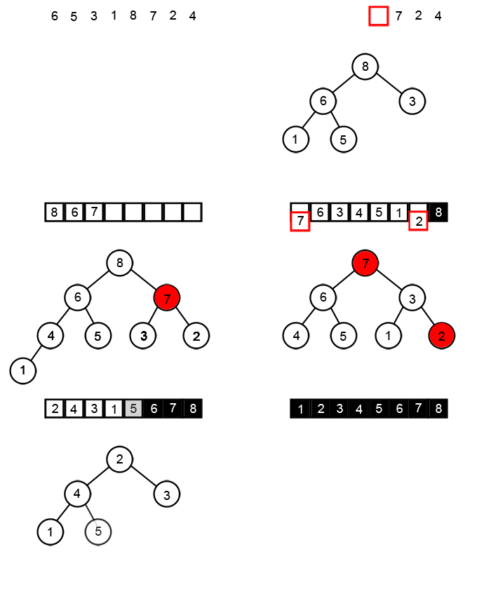
Let’s do some heap sorting!

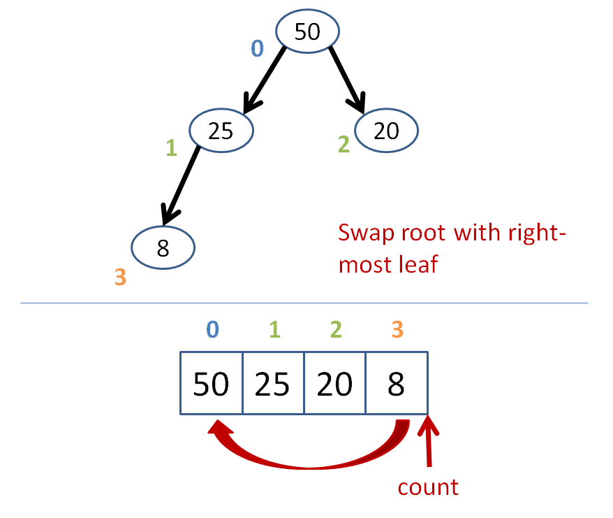
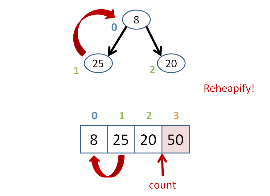
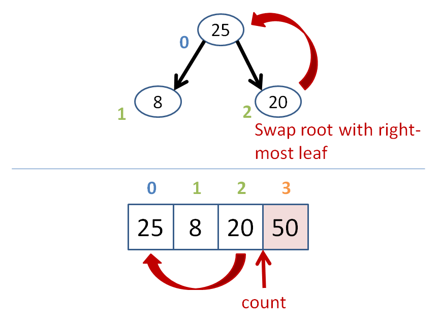
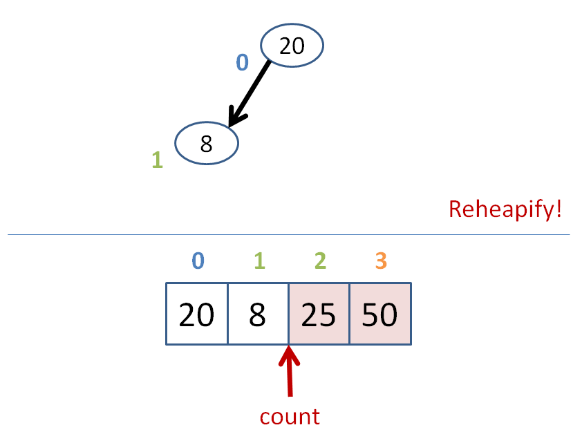
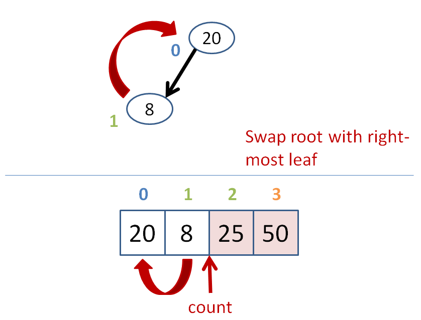
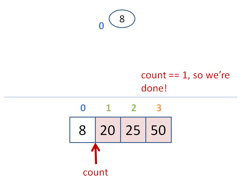
What is the time complexity of heapsort?

For each of n items: getting the largest takes $O(1)$, and popping + reheapifying takes $O(log(n))$. As such, HeapSort exhibits a best, worst, and average case performance of $O(n\ast log(n))$.

How exciting! That looks a lot better, on average, than InsertionSort, even though Insertion can win in the best case.

We see that these two sorting algorithms are similar insofar as they maintain a sorted sub-list that grows incrementally until we are left with a sorted version of the original list.

Here’s a cool animation of that shamelessly stolen from Wikipedia:

Better Sorting

By now, we’ve seen a couple of different sorting algorithms:

• InsertionSort: Worst case $O(n^2)$, Best case $O(n)$
• HeapSort: All cases (for general sorting) $O(n\ast log(n))$

Both of these algorithms belong to the category of reduce-and-conquer since, at every step, they reduce the number of elements required to still be sorted by 1.

Although done in different orders (InsertionSort by locking the first items at the front of the list in place, and HeapSort vice versa), they belong to this same algorithmic paradigm.

Perhaps, however, we can take the idea of “reduce-and-conquer” and think about approaches that, rather than having steps which leave them with slightly smaller subproblems to solve, instead leave them with much smaller ones.

We’ll take a look at a couple of such sorting algorithms now, and at the end, examine a few other important properties of sorting algorithms.

MergeSort

Divide-and-Conquer algorithms recursively divide a large problem into two or more related, smaller subproblems until those subproblems are easy enough to solve directly. The solutions to these smaller subproblems are then somehow recombined to solve the original, larger one.

MergeSort is a divide-and-conquer sorting algorithm that breaks a large list into smaller and smaller sub-lists half their size that are easy to sort, and then recombines the small lists to produce a final, sorted list.

Its performance stems from the following insights.

The Merge Operation

In the context of MergeSort, the merge(list0, list1) operation, given two sorted lists 0 and 1, produces a sorted list out of the elements of both combined.

Let’s see why this might be desirable…

Example

Consider the result of merging the following lists:

• merge([7], [5])
• merge([1, 4, 5, 7], [0, 2, 3, 6])

In the worst case, how many comparisons need be made to sort the 1-item lists? What about asymptotically for 2 x 1-item lists?

A single comparison! O(1) in general.

Interesting… so sorting 2 tiny lists is super easy… put a pin in that insight.

In the worst case, how many comparisons need be made to sort the 4-item lists? What about asymptotically for 2 x n-item lists?

Well, every time we’d need 8 comparisons for the 4 item lists! O(n) in general.

Note: when merging the lists above, we needed an extra storage location that we'll call the workspace that holds the sorted sublist at the end of the merge.

This extra tax on space can be important when memory is at a premium, but is a trait we’ll look at more in-depth later.

So, given the insights from the above, let’s see if we can put it all together.

MergeSort Algorithm

[Reflect] Before reading on, consider how we might combine the algorithmic pieces above into a sorting algorithm that sorts a full list.

Done reflecting? Here are its steps, in a very small nutshell:

1. Take the initial, unsorted list and recursively halve it until we are left with lists containing a single element.
2. Merge these smaller lists into sorted lists twice their size until we are left with a list the size of the original list. This final list will be sorted.

More formally, that looks like:

public static void mergeSort(int[] arr) {
    int[] workspace = Arrays.copyOf(arr, arr.length);
    mergeSort(arr, 0, arr.length - 1, workspace);
}
 
private static void mergeSort(int[] arr, int left, int right, int[] workspace) {
    // Base-case: 1 element lists needn't be sorted
    if (left >= right) {
        return;
    }
    
    // Find the middle index of the current sublist
    int mid = (left + right) / 2;
    
    // Sort left half of arr
    mergeSort(arr, left, mid, workspace);
    
    // Sort right half of arr
    mergeSort(arr, mid + 1, right, workspace);
    
    // Merge sorted sublists
    merge(arr, left, mid, right, workspace);
}
 
private static void merge(int[] arr, int left, int mid, int right, int[] workspace) {
    for (int i = left; i <= right; i++) workspace[i] = arr[i];
    int i = left, j = mid + 1, k = left;
    while (i <= mid && j <= right) {
        if (workspace[i] <= workspace[j]) arr[k++] = workspace[i++];
        else arr[k++] = workspace[j++];
    }
    while (i <= mid) arr[k++] = workspace[i++];
}

Note: merge is a function not shown that merges two sorted lists into one sorted list.

Example

Step One: Take the list 6, 5, 3, 1, 8, 7, 2, 4 and show step 1 of Merge Sort, as we decompose the list into smaller parts. How many divisions do we need to make for a list of these 8 elements? How many divisions for a list of n elements?

Example

Step Two: Show the second step wherein we merge the smaller lists into exponentially larger ones until we have the final sorted list. How many steps do we need to merge the final list of 8 elements? How many merge steps to combine the final list of n elements?

MergeSort Runtime Complexity

Our visualization of Step One above is simply a way of thinking about the way that the recursive steps work themselves out; the real computational effort comes from the merge step and the number of times that it’s repeated.

We can think about that actual investment in computational effort from a couple of insights:

Once broken down into the smallest possible sublists, how much work is the merge step taking at each level that follows while recombining?

$O(n)$ since we’re repeating a merge operation $O(n/k)$ for each of k subproblems at each level.

How many levels will there be to perform this merge operation?

$O(log(n))$ since we’re doubling the size of each subproblem at the previous level with each merge.

Visualizing this, we can think about each level’s subproblem size with the amount of work required to merge it:

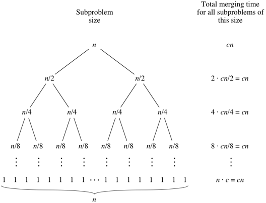Image credit to Khan Academy

So, combining the above observations, what is the asymptotic runtime complexity of MergeSort?

$O(n\ast log(n))$ because we’re repeating the merge operation taking $O(n)$ at each of $O(log(n))$ levels of the MergeSort “tree”.

Visualizations

Let’s take another look at it in action (another gif shamelessly stolen from Wikipedia):

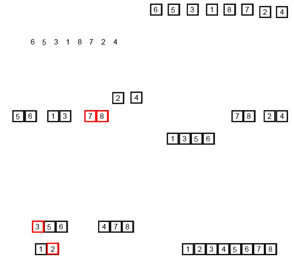
There are some other good MergeSort animations located here.

Quicksort

Quick Sort is another recursive, divide-and-conquer sort that also divides a list into smaller sub-lists using stochastic pivot points.

The sort of choice for the discerning programmer, Quick Sort (or some variant of it) is used in many modern sorting applications. Although it appears to be very similar to MergeSort, we’ll tease out their differences later.

It goes something like this:

# Pseudocode
quicksort (list arr, int begin, int end):
  if end - begin <= 1, return
  randomly choose a pivot index (p), begin <= p <= end
  for each value between begin and end:
	  move values less than arr[p] to left of p
	  move values greater than arr[p] to right of p 
  quicksort(arr, begin, p)
  quicksort(arr, p+1, end)

So, at each call, we choose a pivot randomly, divide the numbers less than and greater than the pivot on either side, then recurse on those sides!

Example

Use QuickSort to sort the following list of ints:

Click here for the steps the algorithm could take. (Gray boxes indicate pivots chosen, orange boxes are left-sublists, and green boxes are right-sublists compared to the pivot)

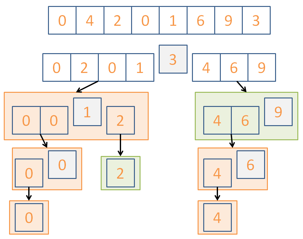
So what is the time complexity of QuickSort?

The average case is that it hits $O(n\ast log(n))$ because of its divide and conquer behavior.

Is QuickSort going to perform equally well every time it runs? If not, what performance can it devolve to?

No! We can get really unlucky with pivot choices and divisions, trending towards O(n^2)

As it turns out, for arbitrary data to sort, it has been proven that $O(n\ast log(n))$ is the best runtime complexity that can be achieved!

There are a variety of improvements to this QuickSort algorithm that better its performance, including:

• Sample values to intelligently pick a pivot (e.g., through median / mean)
• When a sub list is small enough (typically around 9 items) use another sort like insertion sort, then recombine upwards.

Warning: QuickSort performs best when the elements are randomly distributed; a lack of unique values will actually slow it down!

That said, due to smaller constants of proportionality, and the propensity for most data to be heterogeneous, QuickSort is typically heralded as the (name suggesting) empirically quickest sort!

There are some good QuickSort animations located here.

Lomuto Partitioning

Lomuto Partitioning is an algorithmic variant of Quicksort where the pivot is always the last element in the list. (Wikipedia has a good write-up on it here)

The basic argument is this: since a pivot is (in a basic Quicksort) chosen randomly, then any position is an equally viable choice, so might as well choose one that is easy to pivot with.

If we choose the last element as our pivot then:

• We can simply move items less than it to the front of the list starting at the front.
• We can simply shift it over to the left and move items greater than it to the back of the list.

The benefit of Lomuto partitioning is that it gives us a relatively simple algorithm to perform an in-place Quicksort, but we’ll scrutinize its drawbacks shortly…

In the meantime, let’s look at the basic algorithm (credit for this algorithm as listed on the wiki page above, though you can find it pretty much everywhere):

quicksort (arr, begin, end):
	if begin < end:
		p = partition(arr, begin, end)
		quicksort(arr, begin, p - 1)
		quicksort(arr, p+1, end)

# Lomuto Partitioning:
partition (arr, begin, end):
  pivot   = arr[end - 1]                  # Pivot = last element
  swap_ind = begin                        # Swap index starts at beginning
  for j = begin to end - 1:               # For each element in the list...
	  if arr[j] <= pivot:                 # If the current element < the pivot...
		  swap arr[swap_ind] with arr[j]  # Swap the elements
		  swapInd++                       # Then increment the swap index
  swap arr[swap_ind] with arr[j]          # Finally, swap the pivot with the swap index
  return swap_ind                         # And return the pivot's index

Now that we know how it works, let’s see an example:

Example

Use the Lomuto Partitioning Quicksort to sort a small list: 5, 4, 2, 1, 3

arr = [5, 4, 2, 1, 3]
  
# We'll show the first partitioning call:
partition(arr, 0, 4):
s = swap index 
j = iterator
pivot = 3
 
5  4  2  1  3  # arr[j] not < pivot
sj
 
5  4  2  1  3  # arr[j] not < pivot
s  j             
 
5  4  2  1  3  # arr[j] < pivot; swap j, s and then s++
s     j  
 
2  4  5  1  3  # post-swap
 s  j
 
2  4  5  1  3  # arr[j] < pivot; swap j, s and then s++
 s     j
 
2  1  5  4  3  # post-swap
	s  j
 
2  1  5  4  3  # arr[j] not < pivot; j = end - 1, so done iterating
	s  j
 
# finally, swap pivot and s:
2  1  5  4  3
	s
	
2  1  3  4  5  # post-swap
	s
 
# Done with this call to quicksort; now recurse on left half of
# pivot (now at index 2) and right half
quicksort(arr, 0, 1);
quicksort(arr, 3, 4);

Consider: is there a list input format that would cause the Lomuto partitioning approach to have poor performance?

Yes! This algorithm degrades to O(n^2) when the input list is in sorted order or when the list contains all of the same elements!

Can you consider a quick fix that might help with this case?

Randomly choose a pivot element, then swap it with the highest index value (or better yet, sample and choose one a little more intelligently).

Additional Sorting Properties

Alongside the performance analyses that we’ve been conducting with Insertion, Heap, Merge, and QuickSort, there are a variety of other properties of sorting algorithms that we should be careful to dissect.

We’ll look at each of these individually and then close with a summary.

In-Place Sorting

In-Place Sorting Algorithms are those that operate using the memory allocated for the original, unsorted list as the workspace for the sorting operation.

Only one of the algorithms we've seen is not an in-place sorting algorithm; which one is it and why?

MergeSort because the merge operation requires an added auxiliary space to store the intermediary merge results!

Algorithms that do not operate in-place usually come with a memory tax that can be a problem when the sorting task is large, or when memory is at a premium, like on smaller embedded systems.

Stable Sorts

Stable Sorting Algorithms preserve the relative order of items with equal "value" from the pre-sorted format of the list.

To see why this is important, consider sorting objects on multiple field values.

Example

Suppose we are sorting People objects first by First Name, and then by Last Name, and there are two individuals with the same Last Name “Simpson”.

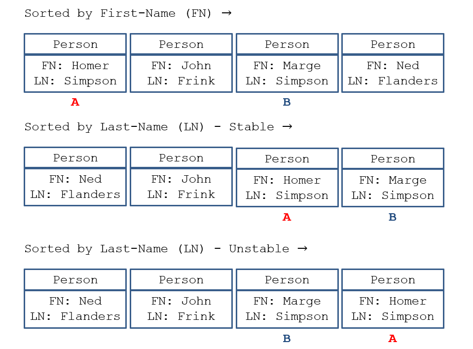
Some notes on the above:

• In the original list, sorted by First Name only, the two with the same last name “Simpson” appear with “Homer” (A) to the left of “Marge” (B).
• If we then wanted to sort by Last Name, but preserve the First Name sorting already performed, we would expect that (A) comes before (B) as well.
• However, since we’re now sorting by a different key (the Last Name), and essentially ignoring the First Name, Stable Sorts will guarantee that (A) is located to the left of (B) just as it was before, but Unstable Sorts may not guarantee that.

What sorting algorithms that we've seen are Stable? Which are not? Why?

The Stable algorithms:

• InsertionSort: given that items being “slid” into place are done in a left-to-right fashion, with swaps being made only between adjacent items, guarantees that items located to the left of others will be sorted before the right ones.
• MergeSort: given that the left sublists are sorted before the right, and then merged in a left-to-right fashion, the relative order of items is preserved.

The Unstable:

• HeapSort: due to reheapification, which can change the relative ordering as the bubble-down process can take an item previously in some right-subtree and sift it down to some left-subtree instead.
• QuickSort: due to the random choice of pivots.

Adaptive Sorts

Adaptive Sorts possess mechanisms for improved efficiency when the list is almost in sorted order.

For many sorting algorithms, this behavior is a natural consequence of the actual sort; for others, making them adaptive comes with some sort of cost.

Are any of our seen sorting algorithms adaptive? Why or why not?

Just InsertionSort! We’ve seen in this case the sorting performance trends to O(n) due to not needing to execute the inner loop.

Of note:

• Because of this reason, there are variants of QuickSort that will actually call InsertionSort on sublists by the time the sublists get small enough.
• Heap and MergeSort also have Adaptive variants, but these come at some additional cost and assumptions that won’t be discussed herein.

And that’s all of the properties we’ve got to cover!

Example

For your own notes: make a table composed of all of our search algorithms, their supported properties, and their best, worst, and average case runtime complexities!