In your latest homework assignment, the spec mentions that a graphical representation is convenient for representing website links, but we should stop to consider
that Graphs themselves are a data type that we can explore!
Graphs are about as fun as a data type can get (if you ask me).
Definition
A graph is an abstract data type consisting of some number of connected Nodes, with fewer restrictions than Trees.
Definition
In graphical terms, we typically call Nodes vertices and the connections between them edges, which can be
either directed (the edge points from one vertex to another) or not.
Such a loose definition! Let’s look at a graph…
Graph Properties
There are many, many graph-analytic properties that depend on their application, but we’ll look at some of the most common now.
Definition
A graph is said to be directed if every edge has at least one directed arrowhead.
This might even mean bidirected arrows with arrows on either end!
Definition
A graph is said to be acyclic if it contains no cycles.
A cycle exists in a graph whenever it is possible, by simply following some path of directed edges, to visit a node twice.
A very common graph representation involves the case where both of these properties are combined:
Definition
A directed, acyclic graph (also known as a DAG) is a directed graph with no directed cycles.
Example
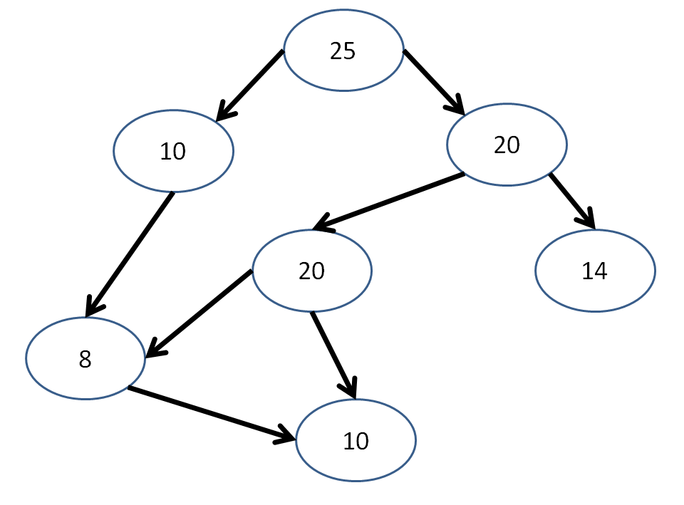
Is the following graph a DAG?
Example
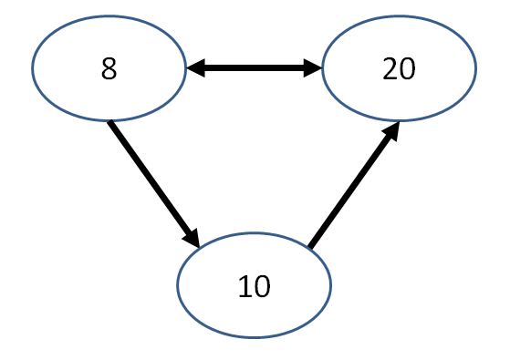
Is the following graph a DAG?
Question
In what scenarios do you think it’s important that graphs are directed and acyclic?
Answer
One example is when temporal ordering is important between vertices (e.g., if A occurs before B in a planning graph, then it’s important
for there to be no cycle like A → B → C → A).
Graph Use-Cases
Now that we’ve seen some simple graphs and their properties, let’s think about when we might use them.
Example
Suggest some possible uses for graphs.
Shortest distances between geographic points.
Mapping social network relationships
Depicting links between websites / Wikipedia Articles
Planning for autonomous agents
Many other AI applications (search, probabilistic reasoning, etc.)
Graphs vs. Trees
Seeing how a graph is just any collection of vertices and edges, let’s think for a second…
Question
Are all trees also graphs?
Answer
Yes! Trees are just graphs with some additional constraints (which we’ll see in a moment).
Question
Are all graphs also trees?
Answer
No! Graphs can have a variety of properties that violate the constraints of trees; let’s see those in the following table.
Graphs vs. Trees
Property
Trees
Graphs
Notion of root
Yes
Not necessarily
One path from root to any node
Yes
Not necessarily
Can contain cycles
No
Yes
Nodes can have multiple inbound arrows
No
Yes
Have methods of traversing nodes
Yes
Yes*
I put a star next to the graph capacity for traversal simply because, unlike with, say, a binary tree, in which we have defined traversal methods like left-to-right postorder, graphs
can be traversed starting at any node and following a variety of different traversal schemas.
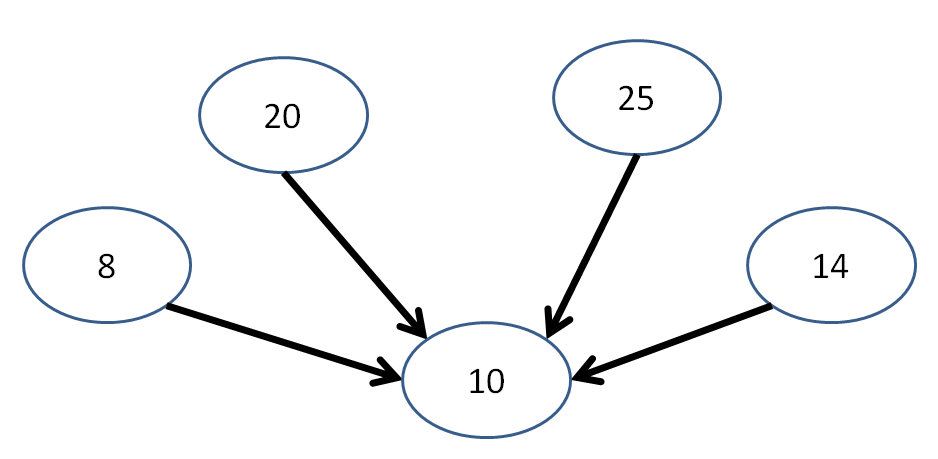
Additionally, we’re not guaranteed that we could traverse all elements of a graph, even if we have a systematic algorithm for doing so. Take the following graph, for example:
Starting at any one of these nodes, we’re not guaranteed that we’ll visit every other node in the graph! (in fact, in this case it’s not possible)
Long story short, there are a variety of niceties we had with trees that are lost with the loose constraints of graphs… but we also gain some cool stuff too.
Graph Traversals
There are a variety of graph traversals for different applications, but for our introduction, let’s just examine 1 or 2.
First, of course, we’ll need some definitions.
Definition
A traversal algorithm provides a procedural means of visiting edge-connected vertices in a graph.
Typically, we use traversal algorithms to process vertices in a graph, or are used in search operations.
Definition
While running, traversals maintain a frontier of vertices it has yet to visit, where the frontier is some DS that facilitates
a traversal order.
Definition
A depth-first traversal of a graph, starting at some vertex V, maintains a Stack frontier that proceeds as follows:
create Stack frontier, Set visitedpush starting vertex onto frontierwhile frontier is not empty: pop vertex U on top of stack if U is in visited: continue visit U and add U to visited set for each child N of U: if N is not in visited: push N onto frontier
Question
Note the “mark V as ‘Visited’” step above; how would you go about accomplishing this efficiently and with clean programming
practices?
Answer
Use a Set to track the collection of already-visited nodes! Note how it would be unwise to store some “visited” field
on the Nodes themselves (if implemented as objects) since we would have to start / end each traversal by reseting that field (computationally wasteful).
Toolkit
Notice a couple key properties about traversals:
The “Depth” first part of this traversal lends itself to the fact that the frontier is a Stack (FILO) and so the most recently added children of any Node
(which are “deeper” from the traversal’s origin) are visited first.
Traversals are not necessarily unique; although we say that we must add all unvisited children of a node to the frontier, this does not specify
a particular ordering of that addition!
Example
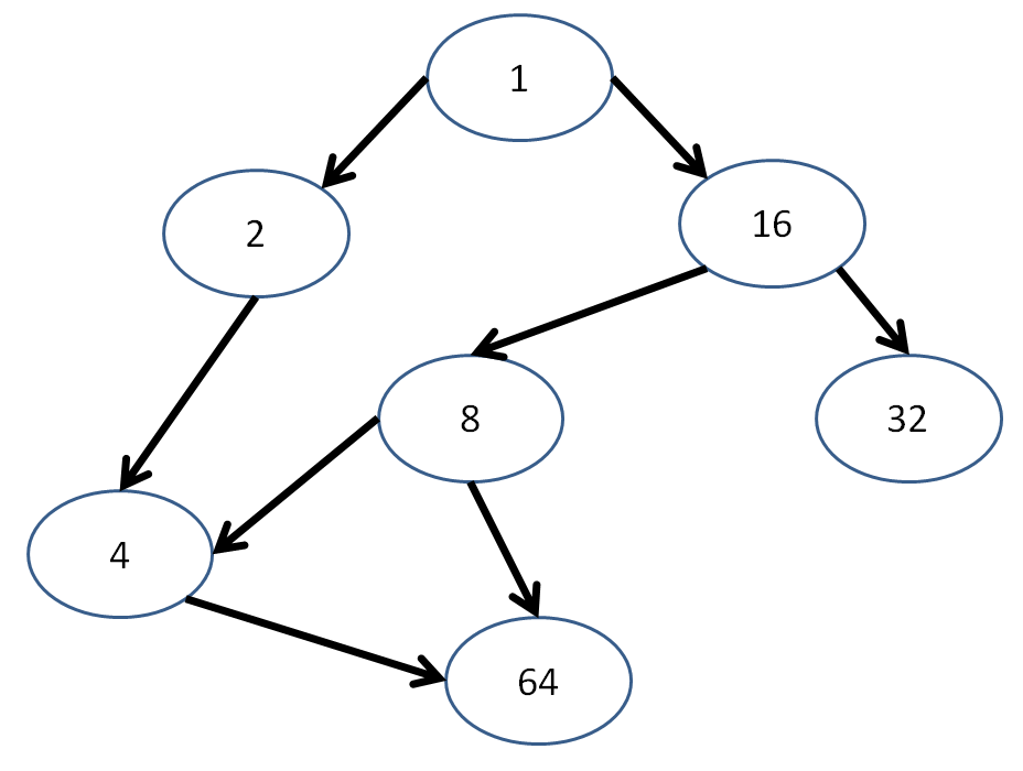
Show a couple of depth-first traversals starting with node 1 in the following DAG:
Some viable depth-first traversals:
1, 2, 4, 64, 16, 8, 32
1, 16, 32, 8, 4, 64, 2
Definition
A breadth-first traversal of a graph, starting at some vertex V, maintains a Queue frontier that proceeds as follows:
create Queue frontier, Set visitedpush starting vertex onto frontierwhile frontier is not empty: pop vertex U at front of Queue if U is in visited: continue visit U and add U to visited set for each neighbor N of U: if N is not in visited: push N onto frontier
This is useful for tracing dependencies where we have to resolve the parents before the children!
Example
What are some viable breadth-first traversals of the following graph?
Why do you think this traversal method is called “breadth first?”
Answer
It visits vertices level by level (breadth) spanning outward from the start vertex.
Representing Graphs
OK cool, but how do we store these graphs? What data structures can we use to represent them?
Definition
The most obvious approach is to use some custom object class where we encode Nodes (vertexes) and Edges (with references to other Nodes) and can
maintain data in either inner-class.
Toolkit
Benefits: Useful when the graph modeled is directed, sparse, and there is extra data to be stored in each Node (e.g., city population where Nodes
are used to model cities on a geographic map).
Problem
Problems: this approach might be overkill if we have only undirected edges or lots of them, or if we’re only using the Nodes to store edges (in which case,
the Node objects may be wasting memory / allocation time)!
Some alternative representations are:
Definition
An adjacency matrix is a 2D array with a row / column for every node, and an indication at index [i][j] of whether node i is connected to node j.
Usually we indicate adjacencies with the number 1 to represent an edge going from node i to node j, and a 0 if there is no edge between them in an undirected graph.
However, we may also use an adjacency matrix when there are both directed and undirected edges by coding, e.g., 2 to represent an undirected
connection, 1 to represent an edge from node i to j, -1 to represent an edge from node j to i.
Example
For example, an adjacency matrix denoting the graph (where each matrix index i corresponds to the node with value 2^i; so, for example, [0][1] corresponds to
the edge from the node with value 1 to the node with value 2) above (with undirected edges instead) might look like:
Benefits: Useful for large, densely connected graphs with potentially directed and undirected graphs.
Remark
Problem: this matrix can have a lot of 0s and waste space when there aren’t many edges in our graph. Also, in general, how to map the nodes to keys,
or more complex data to store in each Node?
Definition
An adjacency map stores each edge connection as a Map of Node keys to Lists / Sets of keys to which that Node is connected.
Example
For example, an adjacency map with integer keys (representing the ints at each node) for the above graph might look like:
Solves the index mapping problem of adjacency matrices while being more memory efficient for more sparse graphs.
Remark
Problem: this adjacency list can be wasteful when our graph has a lot of edges.
Graph Applications
Remark
We won’t have time to examine this section during the present semester, but will see it come back in Algorithms!
Graphs are popularly used to represent geographical data and distances between points (physical or otherwise, in the cases of Networking applications).
For this reason, one of the most ubiquitous graph algorithms helps us compute efficient distances between nodes in a graph.
Definition
Given a graph with vertexes = geographical locations, and edges connecting adjacent locations with some distances between them, Dijkstra’s algorithm tells us the least
distance we would have to travel from a given vertex S to any other vertex in the graph.
Example
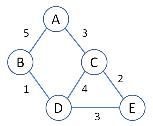
The following example graph lists locations A through E that are separated by distances indicated along the edges.
Question
What is the shorted distance from A to E? What path does it take?
Answer
A → C → E, with a total cost of 5.
Example
Goal: We’d like to have a way of automatically computing the shortest distance from a node to every other node in the network. What are some strategies
you could consider to accomplish this?
Main gist: we want to calculate the minimum distance to get from the start to every vertex in the network in a modified breadth-first fashion so that we always know
the shortest distance to vertex S so that we can then compute the shortest distance from the start to any neighbor of S!
Dijkstra’s Algorithm
Dijkstra’s (one of the most ubiquitous algorithms and, in my opinion, most fun to say) algorithm does precisely the above.
Dijkstra’s algorithm operates by maintaining several data structures:
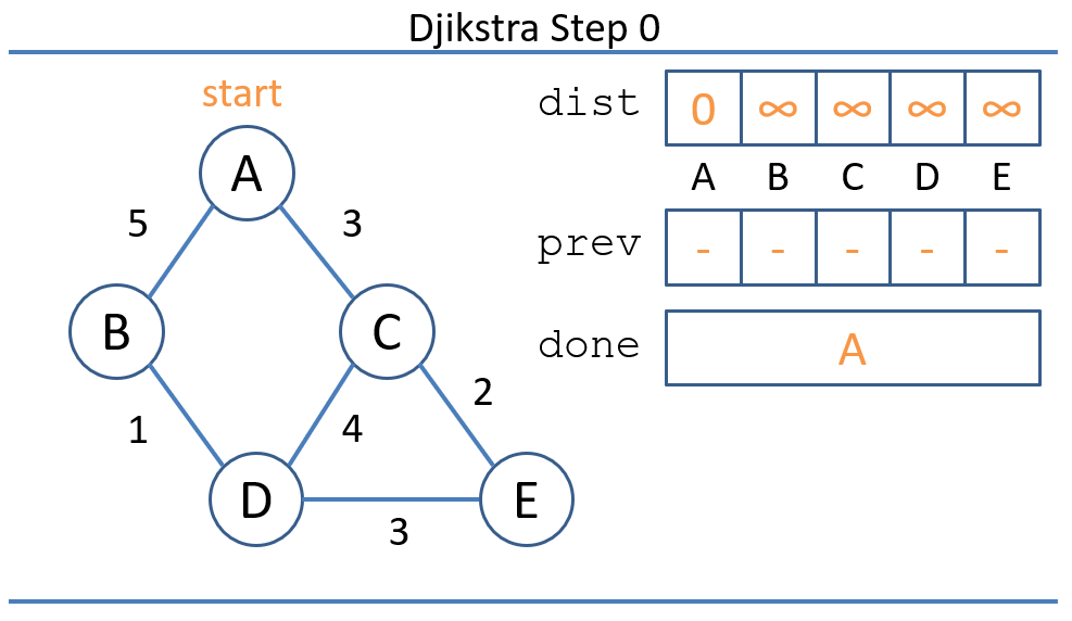
dist: for each node, tracks the optimal distance from the start node. Each element in this vector / map starts out with value infinity, except for the start node, which
starts out with value 0.
done: for each node, tracks whether or not we have already computed the optimal travel distance from it to its neighbors. Implemented as an initially empty
Set.
prev: for each node, tracks the node before this one along the shortest path from the start node.
function Dijkstra(graph, start):
    initialize dist, done, prev (as stated above)
    while done not all true: // Still paths to explore
        u = min distance, not done node from start // track via priority queue
        add u to done
        for each node v in undone neighbors(u)
            d = distance(u, v) // distance between u and v from graph edge
            oldBest = dist[v]
            candidate = d + dist[u]
            if candidate < oldBest
                dist[v] = candidate // Update best distance
                prev[v] = u // Update best path
    return (dist, prev)
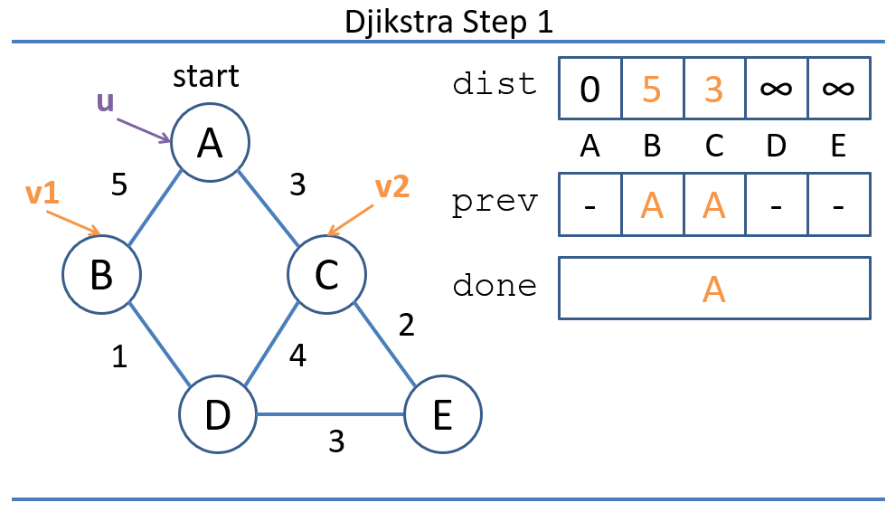
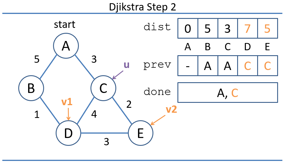
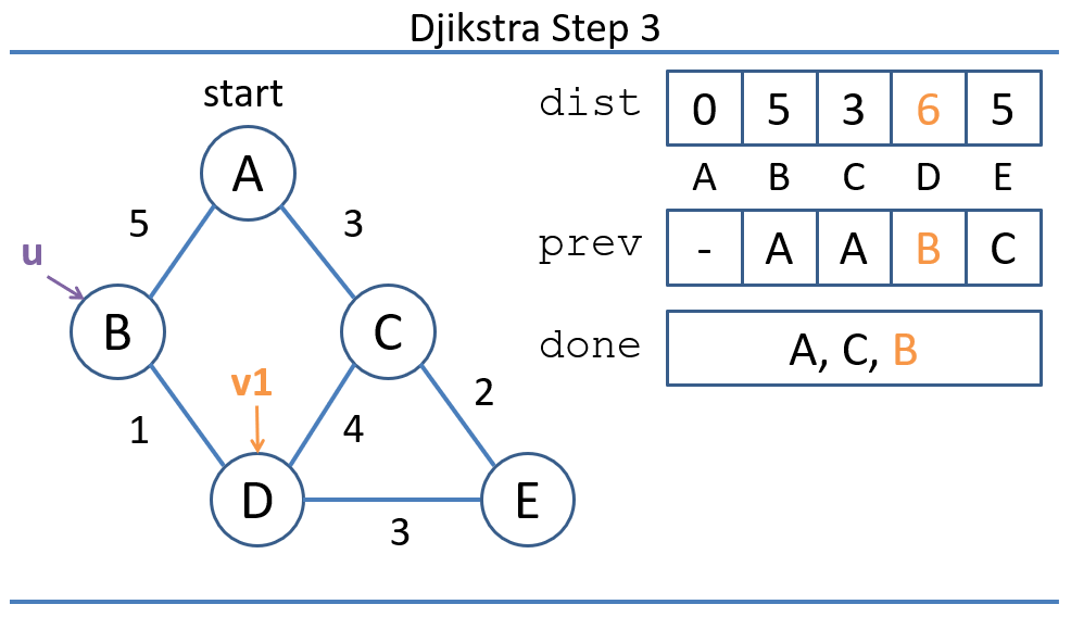
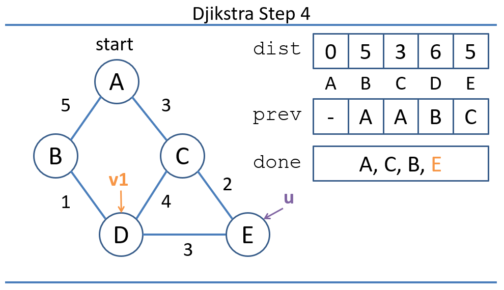
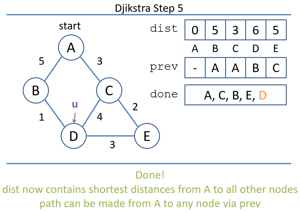
Let’s trace this algorithm through our example now (sorry, forgot to illustrate the prev list below, left as an exercise!).
Question
With the completed dist, prev structures returned from above, how do we find the best path from the source to any destination?
Answer
Just start at the destination’s key / index in prev and walk backwards!
There are many variants of Dijkstra’s algorithm, some suited for different purposes than a general shortest-distance computer, but the gist is the same of each: a procedural way of
finding shortest distances between nodes in a graph.
And that’s Djiksta’s algorithm!
There are variants of the complexity based on the particular implementation, but generally, most vertexes are well connected, and so we have, for |E| = number of edges
in the graph and |V| = number of vertexes, O(|E| + |V|^2), which usually can be proven to be O(|V|^2).